|
Laminar
flow
When a fluid flows through a tube,
e.g. a catheter, the fluid
velocity will be higher in the center of the tube than along
the
wall. This is due to friction. Assuming there is only an axial movement
along the tube the fluid can be modeled as a number of thin, concentric
layers of fluid, where the outermost has a friction against the wall,
the second outermost has a friction against the outermost layer etc.
Layers can be called lamina, and this type of flow is called laminar
flow.
The velocity profile with laminar flow
can be proven to be quadratic using Poiseuille's
law. A useful expression for the velocity profile is:
(Equation 1)
Note that if velocity is
time-invariant a simple multiplication with
a (constant) time will give an expression for the travelled distance
for a particle distance r from the center of the tube, and assuming
constant tube radius (R) a multiplication with the tube cross section
will give the same expression for volume.
Implications
for infusion and sampling
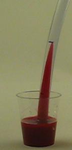
Now, assume the tube is filled with
solvent (e.g. water) and at one
end of the tube there is a solution with concentration C. The solution
is infused into the tube (or withdrawn in the sampling case) causing
the concentrated solution form a paraboloid in the solvent. This
behaviour can be easily shown with a piece of
tube, one transparent and one colored solution. A
hint is to
use a viscous fluid like thick syrup.
A cross section in the tube will be
two coaxial circles - a
concentrated in the center and an outer with zero concentration. The
average concentration in a cross section can be computed as the
fraction of the inner circle divided by the total cross section, i.e.
(Equation 2).
Inserted in eq. 1 with velocity
replaced by volume and some rearranging leads to:
thus average concentration decreases
linearly with (volumetric) distance in tube. Obviously Vmax
= 2V, where V is the volume of solution (B) infused
into the solvent (A) filled tube:
Now
where does this lead us?
When we infuse or withdraw a solution
into a tube, the concentration
is 100% at the source, 50% at the volume pumped and 0% at
twice
the volume pumped. Opposite: with a catheter of 100 µl:
- After pumping 50 µl the solution
reaches the far end, starting at 0% increasing.
- After 100 µl there will be
50% at the far end
- After 200 µl there will be
75% at the far end
- There will (theoretically) never be
100% solution at the far end of the catheter.
The following diagram describes the
effect (V = Volume pumped, L = volumetric length of catheter):
|
Effects
of radial transport
Pure laminar flow deals only with
axial flow. If there is radial
mixing between the solution and the solvent the tip of the paraboloid
will be smeared out across the cross section, and although the fluid
moves with the same speed as in laminar flow the concentration will be
lower at the edge. The effect is that the transition from
unconcentrated to concentrated solution becomes shorter/steeper.
For low fluid velocities and thin
tubes diffusion will contribute to
the radial transport. The subject is well covered in the article Dispersion
of soluble matter..., G.I. Taylor 1953. Not free
unfortunately.
At high velocities the fluid will be
turbulent as opposed to
laminar, i.e. the flow contains vortexes mixing the fluid radially. The
effect will be similar to the difusion case but harder to analyze
mathematically. Taylor wrote another article on the turbulent case: Dispersion
of Matter in Turbulent flow.... For catheters the speed will
rarely be high enough to create a turbulent flow.
In effect, instead of a linear
concentration decay the concentration
will form an erf-shaped transition along the tube. Here is a diagram
for a 0.4 mm catheter at various speeds:
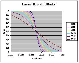
Water self diffusion coefficient is
used. For larger molecules or
more viscous media, coefficient of diffusion will be lower and the
gradient more linear.
Note that the above diagram does not
asymptotically resemble the
laminar flow case. This is due to Taylors assumption that the
length of te tube is much longer than the transition length.
Note also that for very low flow there
will be an axial diffusion
component, so there is a limit to how steep the transition can be. For
infusion/sampling situations this has no practical meaning to my
knowledge.
How
to use this
Theory
is reciprocal so the same model applies
indpendent on whether we withdraw a sample or infuse a drug. The model
does not consider fluids with different viscosity like blood pumped
into a saline-filled catheter (blood has 3-4 times higher viscosity
than saline), but from practical experiments we still have reasonably
good match between theory and practice. Mixing entirely different
fluids like glycerol and water doesn't look like laminar flow at all
(viscosity differ by a factor 10000).
Typically we use low flows
for continuous infusion into rodents
and for classical microdialysis. In these cases we can estimate the
concentration with a steep increase at the pumped volume.
For larger animals we may need to
consider laminar flow model for
continuous infusion. Wider catheters and higher flows reduce the radial
mixing making the gradient slower.
For bolus dosage and faster sampling,
e.g. blood sampling laminar flow model must be considered even for
rodents.
Laminar flow with Taylor-dispersion
(due to diffusion) is tricky
since we often don't know the properties of the solution, i.e.
coefficient of diffusion. Blod for example is a mixture of small
molecules like NaCl, fatty acids, proteins and blood cells, each with
their properties. Heavy particles like erythrocytes are also affected
by gravity which isn't accounted for in the model.
On the positive side, the laminar flow
model without diffusion
describes the worst case scenario, and is very easy to calculate. For a
better model start with an experiment and use the concentration
achieved there.
Finally I would like to
present two diagrams for bolus infusion
(no calculations here) based on the pure laminar model. B is the bolus
volume, L is the catheter volumetric length and V is the flush volume:
|